The dendrites are the receivers of the signal and the axon is the transmitter. Alone, a neuron is not of much use, but when it is connected to other neurons, it does several complicated computations and helps operate the most complicated machine on our planet, the human body. There are inputs to the neuron marked with yellow circles, and the neuron emits an output signal after some computation. The input layer resembles the dendrites of the neuron and the output signal is the axon.
Each input signal is assigned a weight, wi. This weight is multiplied by the input value and the neuron stores the weighted sum of all the input variables. These weights are computed in the training phase of the neural network learning through concepts called gradient descent and backpropagation, we will cover these topics later on. An activation function is then applied to the weighted sum, which results in the output signal of the neuron.
Now let’s implement it on our Trading Agent
The input signals are generated by other neurons, i. This is the basic idea of a neural network. We will look at each of these concepts in more detail in this neural network tutorial. We will look at an example to understand the working of neural networks. The input layer consists of the parameters that will help us arrive at an output value or make a prediction.
Our brains essentially have five basic input parameters, which are our senses to touch, hear, see, smell and taste. The neurons in our brain create more complicated parameters such as emotions and feelings, from these basic input parameters. And our emotions and feelings, make us act or take decisions which is basically the output of the neural network of our brains. Therefore, there are two layers of computations in this case before making a decision. The first layer takes in the five senses as inputs and results in emotions and feelings, which are the inputs to the next layer of computations, where the output is a decision or an action.
Hence, in this extremely simplistic model of the working of the human brain, we have one input layer, two hidden layers, and one output layer. Of course from our experiences, we all know that the brain is much more complicated than this, but essentially this is how the computations are done in our brain.
Reinforcement Learning for Trading Strategies
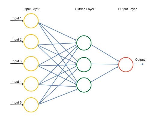
To understand the working of a neural network in trading, let us consider a simple stock price prediction example, where the OHLCV Open-High-Low-Close-Volume values are the input parameters, there is one hidden layer and the output consists of the prediction of the stock price. In the example taken in the neural network tutorial, there are five input parameters as shown in the diagram.
The hidden layer consists of 3 neurons and the resultant in the output layer is the prediction for the stock price. The 3 neurons in the hidden layer will have different weights for each of the five input parameters and might have different activation functions, which will activate the input parameters according to various combinations of the inputs.
For example, the first neuron might be looking at the volume and the difference between the Close and the Open price and might be ignoring the High and Low prices. In this case, the weights for High and Low prices will be zero. Based on the weights that the model has trained itself to attain, an activation function will be applied to the weighted sum in the neuron, this will result in an output value for that particular neuron. Similarly, the other two neurons will result in an output value based on their individual activation functions and weights.
Finally, the output value or the predicted value of the stock price will be the sum of the three output values of each neuron. This is how the neural network will work to predict stock prices. Now that you understand the working of a neural network, we will move to the heart of the matter of this neural network tutorial, and that is learning how the Artificial Neural Network will train itself to predict the movement of a stock price.
To simplify things in the neural network tutorial, we can say that there are two ways to code a program for performing a specific task. The second process is called training the model which is what we will be focussing on. The neural network will be given the dataset, which consists of the OHLCV data as the input, as well as the output, we would also give the model the Close price of the next day, this is the value that we want our model to learn to predict.
The training of the model involves adjusting the weights of the variables for all the different neurons present in the neural network. The cost function, as the name suggests is the cost of making a prediction using the neural network. There are many cost functions that are used in practice, the most popular one is computed as half of the sum of squared differences between the actual and predicted values for the training dataset.
The way the neural network trains itself is by first computing the cost function for the training dataset for a given set of weights for the neurons. Then it goes back and adjusts the weights, followed by computing the cost function for the training dataset based on the new weights. The process of sending the errors back to the network for adjusting the weights is called backpropagation. This is repeated several times till the cost function has been minimized.
We will look at how the weights are adjusted and the cost function is minimized in more detail next. The weights are adjusted to minimize the cost function. One way to do this is through brute force. Suppose we take values for the weights, and evaluate the cost function for these values. When we plot the graph of the cost function, we will arrive at a graph as shown below.
- Stock prediction using recurrent neural networks.
- skills covered?
- forex pending order strategy.
- Neural Networks Learn Forex Trading Strategies.
- A New Approach to Neural Network Based Stock Trading Strategy;
- Using Deep Neural Networks to Enhance Time Series Momentum - QuantPedia.
This approach could be successful for a neural network involving a single weight which needs to be optimized. However, as the number of weights to be adjusted and the number of hidden layers increases, the number of computations required will increase drastically. For this reason, it is essential to develop a better, faster methodology for computing the weights of the neural network. This process is called Gradient Descent. We will look into this concept in the next part of the neural network tutorial.
Neural Network In Python: Introduction, Structure And Trading Strategies
Gradient descent involves analyzing the slope of the curve of the cost function. Based on the slope we adjust the weights, to minimize the cost function in steps rather than computing the values for all possible combinations. The visualization of Gradient descent is shown in the diagrams below. The first plot is a single value of weights and hence is two dimensional. It can be seen that the red ball moves in a zig-zag pattern to arrive at the minimum of the cost function.
In the second diagram, we have to adjust two weights in order to minimize the cost function. Therefore, we can visualize it as a contour, as shown in the graph, where we are moving in the direction of the steepest slope, in order to reach the minima in the shortest duration. With this approach, we do not have to do many computations and as a result, the computations do not take very long, making the training of the model a feasible task.
In batch gradient descent, the cost function is computed by summing all the individual cost functions in the training dataset and then computing the slope and adjusting the weights. In stochastic gradient descent, the slope of the cost function and the adjustments of weights are done after each data entry in the training dataset. This is extremely useful to avoid getting stuck at a local minima if the curve of the cost function is not strictly convex.
Each time you run the stochastic gradient descent, the process to arrive at the global minima will be different. Batch gradient descent may result in getting stuck with a suboptimal result if it stops at local minima. The third type is the mini-batch gradient descent, which is a combination of the batch and stochastic methods.
1 Introduction
The state of the art either employs a deterministic scheme the literature entries using deep learning or very complex evolutionary algorithms for trading rule generation the papers using other machine learning techniques for prediction. The paper is structured in the following manner. Section 2 begins with the description of the novel data collection and draws the conceptual premises for the subsequent modelling.
The chosen deep architectures and the proposed heuristic-driven search strategy are outlined against the state of the art. The experimental part, found in section 3, is composed of the exploration of the best parameter settings, the results of the two deep models and the effect of their predictions within the HC-powered trading strategy on the hypothetically generated profit.
The discussion is concluded in section 4, by also advancing directions for further improvement. The new data employed in this study is described in detail both as concerns its content and the means to access it. The methodology is outlined with respect to the state of the art in deep learning for stock price prediction. The data used refers 25 companies listed under the Romanian stock market.
Neural networks: Where are they now? | Futures
The trading indicators are the number and value of transactions, the number of shares, the minimum, average and maximum prices, the open and close price. The data has been collected since October 16 until March 13 The period for which each business is listed is different, as triggered by the date of the enlisting of the company, as well as the cease of activity at the other end. Fig 1 shows the available history for each of them. The overall trend for the close price as well as an indication of the periods in which this was recorded are illustrated in Fig 2.
The prediction in this study targets only the close price. According to the terminology in [ 2 ], the window length is thus equal to N , the rolling window is equal to 1 day and the predict length also to 1 day.
- Neural networks, the future of trading?.
- tributacion stock options 2017.
- forex pulse detector review.
- Indicators and Strategies.
- forex arbitrage opportunities;
- best martingale ea forex.